S-parameter Viewer: Overlay Touchstone Files and Score KPIs

S-parameter Viewer is a VNA-style plotter for measured Touchstone and MDIF. Files stay in the browser. Drop one .s2p and you get log-mag, phase, VSWR, and group delay with markers. Drop several, and Analysis adds a kind-aware KPI table, an optional datasheet spec, and — when filenames include Unit-N — part-to-part mean, $\sigma$, and pk-pk.

The screenshots use five Mini-Circuits BFCG-252+ lab files (lot Q23590 / EH20353 / 100120) as a stand-in. Same job for any vendor .s1p / .s2p / MDIF.

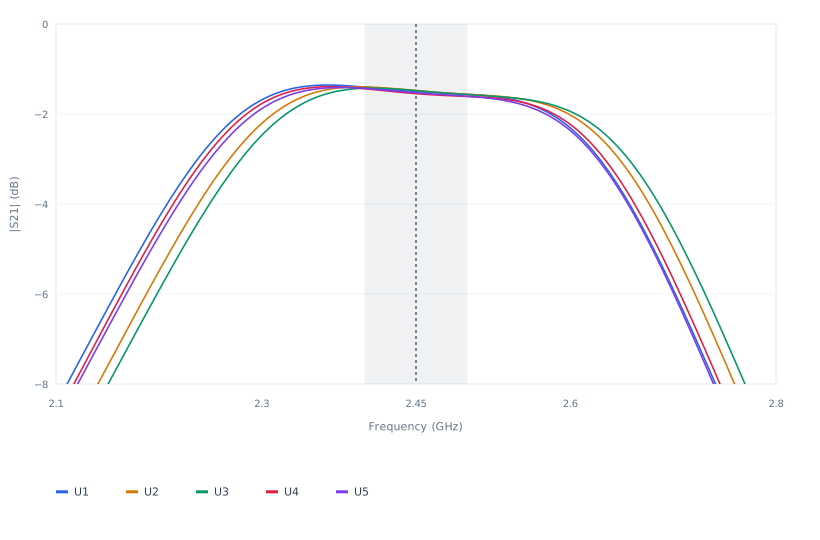
The plots on this page are static copies of that Analysis view, not a live embed. Open the files on /sparam to move the marker and change the band.

Drop files, then pick the band

From S21 the file is classified as an amplifier, filter, equalizer, or generic network. That choice sets the default plot layout and the Auto X window.

For a filter, Auto X is a padded 3 dB band from the peak, snapped to 100 MHz. On the example files that lands at 2.2–2.7 GHz. The datasheet window we will score against is 2.40–2.50 GHz. IL, ripple, return loss, group-delay ripple, and stopband rejection are computed over the analysis band, not over a hidden datasheet table.

On Unit 1, the two windows disagree:

Window	IL	Ripple	RL	GD ripple
Auto 2.2–2.7 GHz	$2.32\,\mathrm{dB}$	$4.537\,\mathrm{dB}$	$3.052\,\mathrm{dB}$	$321.2\,\mathrm{ps}$
Manual 2.40–2.50 GHz	$1.492\,\mathrm{dB}$	$0.1602\,\mathrm{dB}$	$12.79\,\mathrm{dB}$	$62.86\,\mathrm{ps}$

The Auto numbers include the skirts. For a filter, IL is minus the mean in-band $|S_{21}|$. Widen the band and the mean walks down the edges. Return loss does the same: 3 dB of “RL” is a match at 2.2 GHz, not a fail at 2.45 GHz.

Set Manual start/stop to the spec window before you score a datasheet. Leave Auto on when you want the measured 3 dB width. Hide a file on the left to exclude it.

Kind-aware KPIs and specs

The Analysis KPI table follows the classified kind. Filters show f0, 3 dB BW, fractional BW, IL, ripple, RL, GD ripple, and stopband rejection. Amplifiers show gain min/max/mean, flatness, match, isolation, and K/μ. Equalizers show slope. The companion plot is group delay for a filter, Rollett K for an amplifier.

f0 and 3 dB BW come from the unpadded peak-minus-3 dB crossings on $|S_{21}|$, so they do not change when you shrink the analysis window. IL, ripple, and RL do.

Specs in the sidebar are datasheet limits on those KPIs plus an optional in-band min/max mask on the selected quantity. Yield is the fraction of visible files that pass every enabled spec. Enable IL max $3.5\,\mathrm{dB}$ and RL min $10\,\mathrm{dB}$ against 2.40–2.50 GHz and the example set passes. Enable them against Auto 2.2–2.7 GHz and the same files fail on ripple and RL — because you scored the skirts.

Overlay units, then open Part-to-part

Manual band 2.40–2.50 GHz. Marker 2.45 GHz. Quantity $S_{21}$. KPI rounding matches the Analysis table (4 digits); the marker column matches the part-to-part readout (5 digits).

Unit	S21 @ 2.45 GHz	IL	Ripple	RL	GD ripple
1	$-1.5009\,\mathrm{dB}$	$1.492\,\mathrm{dB}$	$0.1602\,\mathrm{dB}$	$12.79\,\mathrm{dB}$	$62.86\,\mathrm{ps}$
2	$-1.478\,\mathrm{dB}$	$1.478\,\mathrm{dB}$	$0.164\,\mathrm{dB}$	$13.71\,\mathrm{dB}$	$85.72\,\mathrm{ps}$
3	$-1.4793\,\mathrm{dB}$	$1.486\,\mathrm{dB}$	$0.1446\,\mathrm{dB}$	$13.72\,\mathrm{dB}$	$106.2\,\mathrm{ps}$
4	$-1.5477\,\mathrm{dB}$	$1.537\,\mathrm{dB}$	$0.1729\,\mathrm{dB}$	$12.63\,\mathrm{dB}$	$51.87\,\mathrm{ps}$
5	$-1.5266\,\mathrm{dB}$	$1.522\,\mathrm{dB}$	$0.1748\,\mathrm{dB}$	$13.45\,\mathrm{dB}$	$53.1\,\mathrm{ps}$

Datasheet typical at 2450 MHz is 1.50 dB IL and 12.83 dB RL. Unit 1 is that file, to rounding.

The Units tab runs when two or more files parse a unit id. Name them filter_Unit-1.s2p or put DATA FOR:Unit 1 in a comment. Mini-Circuits already does both.

At 2.45 GHz this five-unit overlay reports:

	S21
Mean	$-1.5065\,\mathrm{dB}$
$\sigma$	$0.030354\,\mathrm{dB}$
pk-pk	$0.06972\,\mathrm{dB}$
min (U4)	$-1.548\,\mathrm{dB}$
max (U2)	$-1.478\,\mathrm{dB}$

Mean insertion loss at the marker is $1.5065\,\mathrm{dB}$. That is the number to put in a cascade budget for this lot, not the 1.7 dB typical line.

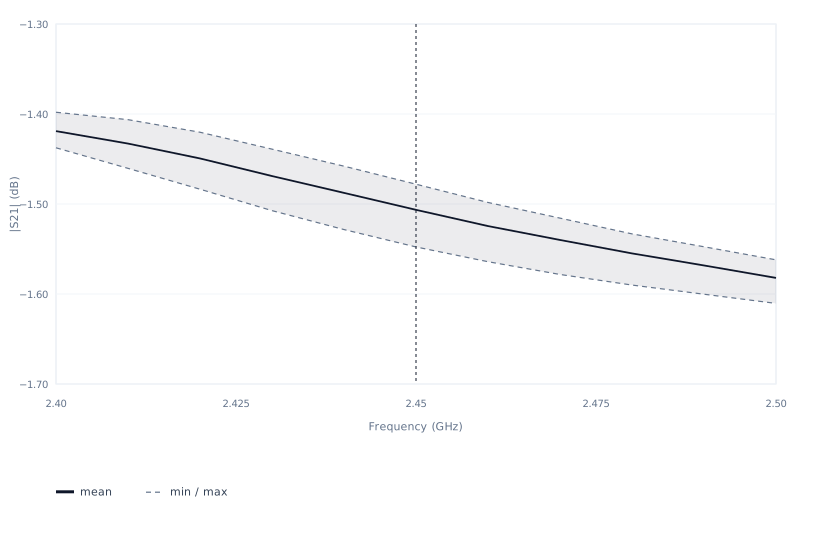
The envelope is min / mean / max versus frequency on a common grid. An in-band min/max mask on the selected quantity scores yield; Cp/Cpk appears only when the mask has both sides. Five parts is a lot overlay, not a process study.

Temperature Δ is a third Analysis tab. It wants +25C or Temp: 25C in the name. The example files have none; the temperature note uses the EQY set.

What to change

Keep Unit-N in the filename. Drop your own set on S-parameter Viewer.

1. Confirm kind (filter, amplifier, equalizer) and whether Auto X is the band you meant.
2. Switch Analysis to Manual if you are scoring a datasheet window. In the example that is 2.40–2.50 GHz, marker 2.45 GHz.
3. Read the KPI table, then open Part-to-part for mean, $\sigma$, and pk-pk.
4. Switch quantity to $|S_{11}|$ or S21 GD if that is the spec you bought. Enable a spec or a mask to score yield.

When a typical file is enough

A single eval-board .s2p is the right first-pass number for a cascade sketch. Overlay the lot when insertion loss is your margin, you are buying to a max spec, or you are about to copy “typical” into a Monte Carlo that is supposed to be unit-to-unit.

This set’s 0.06972 dB pk-pk is not a license to ignore a 3.5 dB max on the next date code.

What this is not

S-parameter Viewer is a browser plotter, not a VNA and not a cascade or mismatch solver. Group delay is from unwrapped S21 phase. Auto 3 dB edges are interpolated from the sampled grid; they are not a fitted filter model. Export CSV needs a signed-in IndieRF account; viewing does not.

The scalar cascade in RF Cascade Analyzer still treats a filter as loss/NF at one frequency. It does not ingest these .s2p files as a two-port.