Validation

How IndieRF checks its numbers

Seventeen checks, one per tool, hold IndieRF's results to an answer worked outside its code: scikit-rf for Touchstone files, schematic circuits, the VSWR table, attenuator pads, stability circles, amplifier gains, matching chains and coax SWR; hand math for the cascade, op-amp templates and dB ratios; independent Python for transmission lines, the link budget, mixer spurs and phase noise to jitter; known data for the plot digitizer; and solves of the same box and openEMS for Planar EM. Every count on this page is read from the tests' own fixture files when the site is built, so the page and the tests cannot disagree.

A share link holds the whole design

A Cascade or Schematic share link carries the whole design, compressed into the part of the link after the #. It does not point to a saved copy on a server, so opening it needs no account, database or cloud project: only the IndieRF page to read it. Links from the Transmission Line, Coax Loss, dB Converter and Smith chart tools carry their typed inputs in the link the same way.

Cloud saves are different: they live on IndieRF's servers and need sign-in. A Schematic that uses data files gets a .zip in place of a link, because file bytes never go in a URL.

RF Cascade Analyzer

Cascade gain, NF, IP3, P1dB and SFDR against hand math

Checked
29 chain-output values from 10 line-ups: gain, noise figure, IIP3, OIP3, input P1dB, output P1dB and SFDR. Each line-up runs through the same solver and path metrics the canvas uses.
Reference
Worked by hand from the textbook equations (Friis, and the reciprocal sums for intercept and compression), never by running the engine. 6 of the 10 cases follow a published example or a vendor calculator's formulas; the derivation for each is in the fixture file.
Tolerance
0.005 dB and 0.05 dB absolute, set per case.
Result
29 of 29 values match. No known discrepancy is pinned.
Does not cover
A matched, one-way scalar chain of amplifiers and losses. Mismatch between stages, filter shape, IM2, and the branching, combining, mixer and ADC nodes are outside these cases.
Test files
  • lib/cascade/golden-fixtures.ts
  • lib/cascade/__tests__/golden/golden.test.ts
The cases and their sources
  1. Lossy line followed by an amplifier (Pozar noise example). Pozar, Microwave Engineering, 4th ed., Ch. 10, Example 10.3 (lossy line, then amplifier); Eq. for a lossy line F = 1 + (L - 1) T / T0 and Friis cascade F = F1 + (F2 - 1) / G1. Source page
  2. Three-stage LNA, filter, mixer noise figure. Friis cascade, Pozar, Microwave Engineering, 4th ed., Sec. 10.1: F = F1 + (F2 - 1)/G1 + (F3 - 1)/(G1 G2).
  3. Cascaded IIP3 and OIP3, LNA, filter, mixer. Reciprocal input-referred intercept sum, Pozar, Microwave Engineering, 4th ed., Ch. 10 (intermodulation of cascaded stages); 1/IIP3 = 1/IIP3_1 + G1/IIP3_2 + G1 G2/IIP3_3.
  4. Published cumulative IIP3 (MathWorks RF chain example). MathWorks RF Toolbox, rfchain cumiip3 reference page: gains 11, -3, 7 dB; NF 25, 3, 5 dB; IIP3 19, Inf, 3 dBm. Published result about -5.02 dBm. Source page
  5. Single-stage P1dB referred to the input. IP1dB = OP1dB - G + 1 dB, Pozar, Microwave Engineering, 4th ed., Ch. 10 (1 dB compression point); Razavi, RF Microelectronics, Ch. 2.
  6. Cascaded P1dB when one stage dominates. Reciprocal input-referred compression sum, 1/IP1dB = sum of G_prior/IP1dB_k, as used by the Qorvo and TI cascade calculators. Source page
  7. Cascaded P1dB, LNA then mixer contribute comparably. Reciprocal input-referred compression sum, as used by the Qorvo and TI cascade calculators. Source page
  8. Spurious-free dynamic range of a two-stage receiver. SFDR = (2/3) (IIP3 - N_floor), N_floor = -174 dBm/Hz + NF + 10 log10(B). Pozar, Microwave Engineering, 4th ed., Ch. 10 (dynamic range).
  9. Receiver line-up in the Qorvo cascade calculator input form. Qorvo Cascade Analysis Calculator: per-stage gain, NF, P1dB and IP3 in, cascaded NF, OIP3 and P1dB out. Formulas as published on the calculator page. Source page
  10. Receiver line-up in the TI RF cascade calculator input form. TI RF Cascade Calculator: per-stage gain, NF and OIP3 in, cascaded NF and IIP3 out, using the Friis formula and reciprocal intercept sum. Source page

S-parameter Viewer

Touchstone parser against scikit-rf

Checked
2254 complex S values at 256 frequency points in 37 files of up to 8 ports: 16 exports from VNAs and EM and circuit tools (Keysight, Rohde & Schwarz, Ansys HFSS, CST, Cadence Sigrity and AWR, Qucs), 16 examples from the Touchstone 2.0 specification, and 5 files with a zero-ohm reference.
Reference
scikit-rf 2.2.0 reading the same files. Its answers are saved once and committed, so the test needs no Python.
Tolerance
|ΔS| below 10⁻⁹ on every entry. Z0 within 10⁻⁶ Ω.
Result
37 of 37 files match. 2 files with a complex port impedance compare S only, because the viewer holds a real Z0. The mixed-mode example (1 file) is checked against its own rows, because scikit-rf reorders its ports.
Does not cover
Reading the file. Derived quantities (stability K and μ, group delay, return loss), the plots, and MDIF files are tested in other suites, not against scikit-rf.
Test files
  • lib/sparam/__tests__/fixtures/skrf-reference.json
  • lib/sparam/__tests__/vendor-files.test.ts

Plot Digitizer

Plot Digitizer Auto-trace benchmark

Checked
106 plot images run end to end through Auto-trace: plot frame, both axes, legend names and every curve. Most are plots rendered from known data; the datasheet scans are scored on their axes and curve count.
Reference
The values each plot was drawn from, or for a scan its printed axes, kept apart from the tool's code.
Tolerance
A case passes when every axis is confirmed within 1% of span, every curve is found within 1% of span with its legend name, and no extra curve comes back.
Result
93 of 106 pass, and 0 confirmed an axis more than 1% off. Each of the 13 that fail is listed in the test with its reason. These are the last full bench run with live Tesseract OCR; the test suite replays its recorded words and fails if a pass turns into a fail or a number gets worse.
Does not cover
Rendered plots and a few datasheet scans. Phone photos of printed pages and hand-drawn curves are outside it, and live OCR in the browser can read a label differently from the recorded words.
Test files
  • lib/grabber/__tests__/fixtures/ocr/summary.json
  • lib/grabber/__tests__/bench-replay.test.ts

Transmission Line Calculator

Edge-coupled microstrip: closed form and field solve

Checked
28 even- and odd-mode values (Ze, Zo, εe, εo) for 3 pairs at 7 geometry and frequency points from the Kirschning–Jansen closed form, and 80 static values for 20 pairs from the 2-D field solve, 12 of them under solder mask.
Reference
Kirschning and Jansen (IEEE Trans. MTT, 1984) worked independently in Python from Wadell's handbook equations. The field solve against a separate Python finite-volume solve meshed to convergence, which reproduces Cohn's exact coupled stripline.
Tolerance
Closed form: Z within 5 × 10⁻⁹ Ω and ε within 5 × 10⁻¹⁰. Field solve: within 0.1% of the reference.
Result
28 of 28 closed-form values and 80 of 80 field-solve values match.
Does not cover
That the code computes the published model. The model's own error against measured boards, and frequency dependence in the field solve (carried to frequency by the closed form), are outside it.
Test files
  • lib/trace-studio/reference-values.ts
  • lib/trace-studio/__tests__/coupled-lines.test.ts
  • lib/trace-studio/__tests__/coupled-fieldsolve.test.ts

RF Schematic Simulator

Schematic engine S-parameters against scikit-rf

Checked
17 circuits at 1518 frequency points, up to 4 ports: pads, LC resonators, a Chebyshev low-pass, lossy lines and stubs, a Wilkinson, Touchstone blocks, hierarchy, and complex port references. Each runs through both the dense and the sparse solver.
Reference
scikit-rf (2.1.0 and 2.2.0) building each circuit with its own Circuit and media classes.
Tolerance
Relative error below 10⁻⁹, or 10⁻¹² absolute where |S| is below 10⁻³. Passive circuits are also checked for reciprocity and passivity.
Result
17 of 17 circuits match with both solvers.
Does not cover
Linear S-parameters. Noise parameters, transistor models and microstrip discontinuities are checked against closed forms worked in Python, in separate engine tests not counted here. Nonlinear analysis is outside it.
Test files
  • engine/crates/rfsim-core/tests/fixtures
  • engine/crates/rfsim-core/src/golden.rs
  • engine/crates/rfsim-core/tests/fixtures.rs

VSWR Converter

VSWR, return loss and mismatch loss against scikit-rf

Checked
392 values in the 56 rows of the VSWR 1.01 to 10 table: |Γ|, VSWR, return loss, |S11| in dB, mismatch loss, and reflected and delivered power.
Reference
scikit-rf 2.2.0 building each row as a real 50·VSWR Ω load on a 50 Ω reference (Network.from_z), with mismatch loss and reflected power from numpy on its |Γ|. Its answers are saved once and committed.
Tolerance
|Γ| and VSWR within 10⁻¹² relative, every dB column within 10⁻⁹ dB, and power within 10⁻⁹ percentage points.
Result
56 of 56 rows match in every column.
Does not cover
A real load on a real reference impedance. Complex reference impedances, the phase of Γ, and mismatch between a source and a load that are both off 50 Ω are outside it.
Test files
  • lib/reflection/skrf-reference.json
  • lib/reflection/__tests__/reflection.test.ts

Planar EM

Planar EM against independent solves of the same box

Checked
20 numbers in 12 cases: lines, a coupled pair, resonators, a series gap, a tee, a bend, a step and wide sections, each solved in the closed metal box Planar EM meshes. The other 66 gated rows of the same table hold the solver to itself: a finer basis, more modes, a moved mesh. Each case also has a convergence study on three or more meshes, with its plot.
Reference
Named with each case: a two- or three-dimensional quasi-static solve of the same box, Cohn's exact stripline, openEMS run offline as reference data, or a published closed form, with the accuracy its source claims.
Tolerance
Set per number, from 0.5% to 2.5% where the gate is relative, and as a difference of S where it is absolute.
Result
86 of 86 gated rows pass on solver 1.3.0. Against openEMS, the step differs by |ΔS| 0.0096 at most, inside the rule of 0.02, and the gap's |Y21| by 3.94%, outside the rule of 2%.
Does not cover
Planar EM is a companion to Trace Studio and the schematic: it cross-checks lines, turns discontinuities into Touchstone files, and sizes stubs and matching sections. These cases are lossless, with zero-thickness metal in a closed box. Conductor loss is shown but not validated, and antennas, vias and thick metal are outside it.
Test files
  • lib/validation/em/golden-table.json
  • lib/em-sim/bench/golden-references.json
  • engine/crates/em-core/src/golden/table.rs
  • lib/validation/em/openems-two-widths.csv
  • lib/validation/em/openems-series-gap.csv
  • lib/validation/__tests__/em-openems.test.ts
  • lib/validation/em/convergence.json
The cases, our numbers and their references
  1. Microstrip line

    Geometry
    A 1.5 mm line on 0.8 mm FR-4 (εr 4.4) under 8 mm of air, 10 mm long, wall to wall, at 1 GHz.
    Reference
    A 2-D quasi-static solve of the same box cross-section, converged to 0.005%, plus the Kirschning-Jansen dispersion increment (published to 0.6%; at 1 GHz the increment is 0.2% of εeff).
    Box and cell
    10 by 12.5 mm, lid 8.8 mm, 50 µm, stop 1 GHz, 111 unknowns
    • Z0: ours 50.42 Ω, reference 50.26 Ω, error +0.32%, gate within 0.5%, pass25 µm cells: 50.32 Ω (+0.11%)
    • εeff: ours 3.295, reference 3.301, error −0.18%, gate within 0.5%, pass25 µm cells: 3.296 (−0.15%)

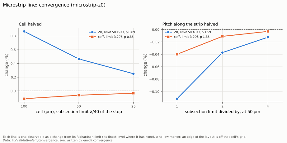
    Z0 on 100, 50 and 25 µm cells: 50.625 Ω, 50.424 Ω and 50.316 Ω. Richardson limit 50.190 Ω, observed order 0.89 where about 1 is expected. Convergence plot

  2. Stripline

    Geometry
    A 1.5 mm strip centred in 1.6 mm of FR-4 (εr 4.4) between the floor and the lid, at 1 GHz.
    Reference
    Cohn's closed form, exact for a zero-thickness strip; εeff is εr exactly.
    Box and cell
    10 by 12.5 mm, lid 1.6 mm, 50 µm, stop 1 GHz, 111 unknowns
    • Z0: ours 32.69 Ω, reference 32.57 Ω, error +0.36%, gate within 1%, pass25 µm cells: 32.61 Ω (+0.12%)
    • εeff: ours 4.398, reference 4.400, error −0.05%, gate within 0.5%, pass25 µm cells: 4.398 (−0.05%)

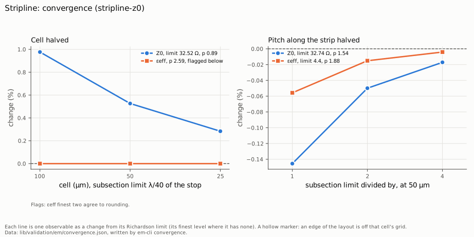
    Z0 on 100, 50 and 25 µm cells: 32.835 Ω, 32.688 Ω and 32.609 Ω. Richardson limit 32.517 Ω, observed order 0.89 where about 1 is expected. Convergence plot

  3. Stripline at 5 GHz, in 50 Ω

    Geometry
    The same stripline, 7 mm long, read as S in 50 Ω at 5 GHz.
    Reference
    Exact: Cohn's Z0 and εeff = εr give S of a 7 mm line in 50 Ω.
    Box and cell
    7 by 12.5 mm, lid 1.6 mm, 50 µm, stop 5 GHz, 189 unknowns
    • |S21|: ours 0.9160, reference 0.9148, error +0.0012, gate within ±0.002, pass
    • |S11|: ours 0.4013, reference 0.4040, error −0.0027, gate within ±0.005, pass

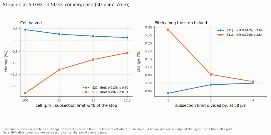
    |S21| on 100, 50, 25 and 12.5 µm cells: 0.9178, 0.9160, 0.9152 and 0.9146. Richardson limit 0.9136, observed order 0.60 where about 1 is expected. Convergence plot

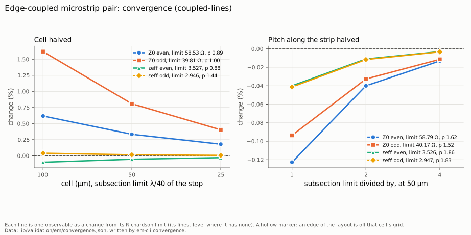
  4. Edge-coupled microstrip pair

    Geometry
    Two 1.5 mm lines 0.4 mm apart on the same FR-4, 10 mm long, at 1 GHz.
    Reference
    A 2-D quasi-static solve of the same box plus the Kirschning-Jansen increment. The open-space Kirschning-Jansen 1984 fit claims about 1%.
    Box and cell
    10 by 14.4 mm, lid 8.8 mm, 50 µm, stop 1 GHz, 222 unknowns
    • Z0 even: ours 58.72 Ω, reference 58.62 Ω, error +0.17%, gate within 1%, pass25 µm cells: 58.63 Ω (+0.02%)
    • Z0 odd: ours 40.13 Ω, reference 39.75 Ω, error +0.96%, gate within 1%, pass25 µm cells: 39.97 Ω (+0.55%)
    • εeff even: ours 3.525, reference 3.535, error −0.29%, gate within 1%, pass25 µm cells: 3.525 (−0.26%)
    • εeff odd: ours 2.946, reference 2.946, error −0.00%, gate within 1%, pass25 µm cells: 2.946 (−0.01%)

    Z0 even on 100, 50 and 25 µm cells: 58.887 Ω, 58.720 Ω and 58.630 Ω. Richardson limit 58.526 Ω, observed order 0.89 where about 1 is expected. Convergence plot

  5. Open-ended line resonance

    Geometry
    A 20.2 mm line from the port wall to an open end, the first series resonance near 2 GHz.
    Reference
    The box line's εeff over the line plus its open-end extension, taken two ways: the Kirschning-Jansen-Koster fit (about 2.5% of the extension, 0.04% of the frequency) and a 3-D quasi-static solve of the same box.
    Box and cell
    25.7 by 12.5 mm, lid 8.8 mm, 50 µm, stop 2.4 GHz, 286 unknowns
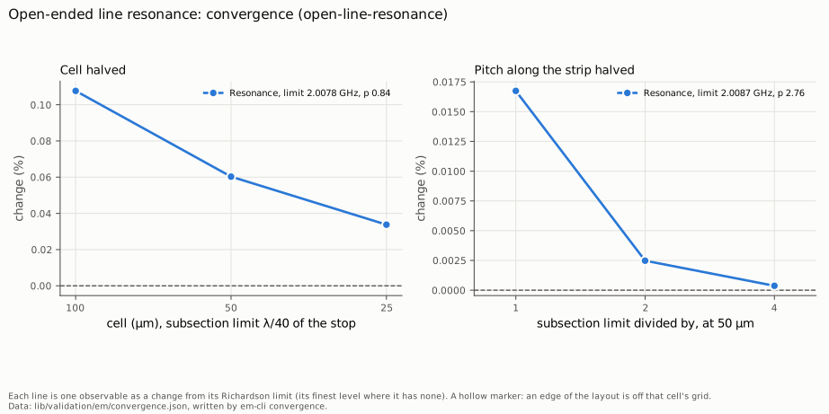
    • Resonance, KJK open end: ours 2.009 GHz, reference 2.007 GHz, error +0.09%, gate within 0.5%, pass
    • Resonance, 3-D open end: ours 2.009 GHz, reference 2.006 GHz, error +0.16%, gate within 0.5%, pass

    openEMS of the same box with a feed in place of the port wall, 3 meshes up to 1.24 million cells: first series resonance 2.009 GHz. Ours is +0.004% from it, against a rule of 0.5%. openEMS moves +0.020% between its two finest meshes.

    Resonance on 100, 50 and 25 µm cells: 2.0099 GHz, 2.0090 GHz and 2.0085 GHz. Richardson limit 2.0078 GHz, observed order 0.84 where about 1 is expected. Convergence plot

  6. Series gap

    Geometry
    Two 5 mm lines, 1.5 mm wide, with a 0.2 mm gap between them, |Y21| at 1 GHz.
    Reference
    A 3-D quasi-static method-of-moments solve of the same box, ±0.3%. Ours is the Richardson value from 50, 25 and 12.5 µm cells. Garg and Bahl's closed form reads 8.4% lower here and is not used.
    Box and cell
    10.2 by 12.5 mm, lid 8.8 mm, Richardson on 50, 25, 12.5 µm, stop 1 GHz
    Cells
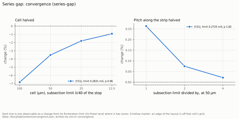
    50 µm 0.2732 mS, 25 µm 0.2780 mS, 12.5 µm 0.2805 mS
    • |Y21|: ours 0.2831 mS, reference 0.2851 mS, error −0.68%, gate within 2.5%, pass

    openEMS of the same layout with no end walls, 4 meshes up to 5.78 million cells: |Y21| 0.2948 mS. Ours is −3.94% from it, against a rule of 2%. openEMS moves +0.11% between its two finest meshes.

    |Y21| on 100, 50, 25 and 12.5 µm cells: 0.26381 mS, 0.27318 mS, 0.27804 mS and 0.28053 mS. Richardson limit 0.28315 mS, observed order 0.96 where about 1 is expected. Convergence plot

  7. Shunt open stub (tee)

    Geometry
    A 1.5 mm through line with a 20.2 mm open stub off its side, the notch near 2 GHz.
    Reference
    Hammerstad's 1981 tee, the open-end extension and the box line's εeff. The tee's reference-plane shift is not well quantified; ±5% of it moves the notch ±0.8%.
    Box and cell
    12 by 32.7 mm, lid 8.8 mm, 50 µm, stop 3 GHz, 1014 unknowns
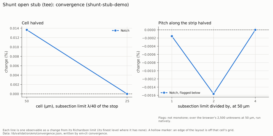
    • Notch: ours 2.036 GHz, reference 2.032 GHz, error +0.19%, gate within 1.5%, pass

    Notch on 50 µm cells with the subsection length divided by 1, 2 and 4: 2.03593 GHz, 2.03591 GHz and 2.03594 GHz. The levels do not move one way and span 0.0016%, so no Richardson limit is given. Convergence plot

  8. Right-angle bend

    Geometry
    A 1.5 mm line that turns 90 degrees in a 10 by 10 mm box, 5 mm arms, |S11| in 50 Ω.
    Reference
    Hammerstad's bend model between two arms of the box line. Its C and L are published to about 5% and 3%.
    Box and cell
    10 by 10 mm, lid 8.8 mm, 50 µm, stop 5 GHz, 536 unknowns
    • |S11|: ours 0.0166, reference 0.0122, error +0.0044, gate within ±0.01, pass

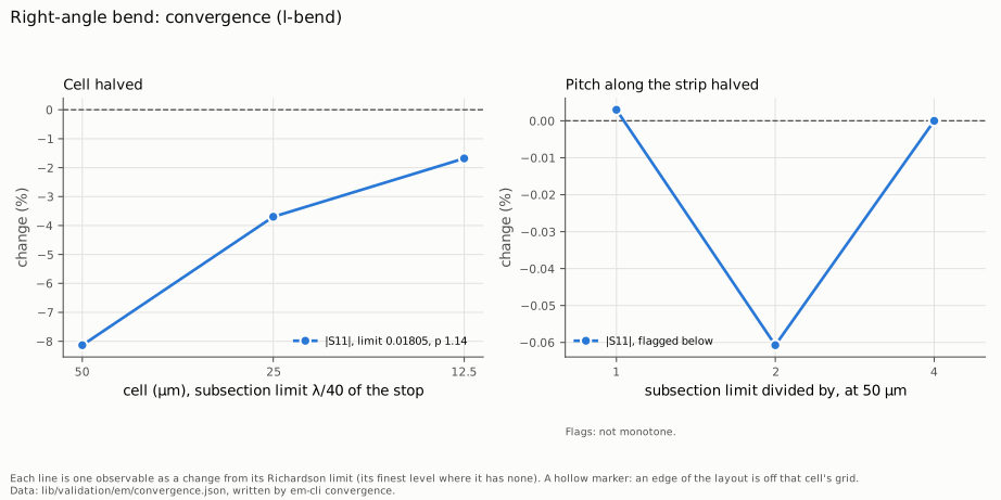
    |S11| on 50, 25 and 12.5 µm cells: 0.01659, 0.01739 and 0.01775. Richardson limit 0.01805, observed order 1.14 where about 1 is expected. Convergence plot

  9. Step in width

    Geometry
    6 mm of 1.5 mm line, then 6 mm of 0.8 mm line, |S21| in 50 Ω at 5 GHz.
    Reference
    Hand model: the two box lines with the Garg and Bahl step (its C about 10%, its L about 5%). openEMS of the same layout below.
    Box and cell
    12 by 12 mm, lid 8.8 mm, 100 µm, stop 5 GHz, 368 unknowns
    • |S21|: ours 0.9521, reference 0.9540, error −0.0019, gate within ±0.003, pass

    openEMS of the same layout with no end walls, 3 meshes up to 2.02 million cells: S11, S21 and S22 at 1 to 5 GHz differ from ours by 0.0096 at most (S22 at 2 GHz), against a rule of 0.02. |S21| is within 0.10% and its phase within 0.23 degrees. openEMS moves 0.0008 between its two finest meshes.

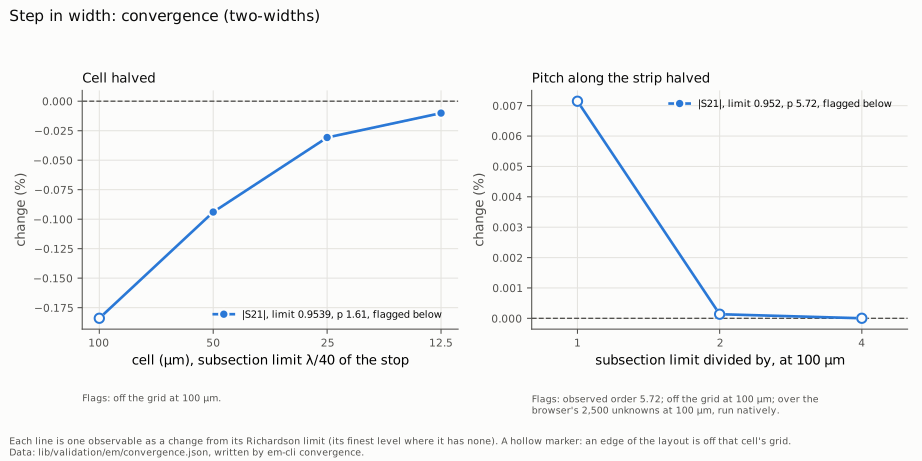
    |S21| on 100, 50, 25 and 12.5 µm cells: 0.9521, 0.9530, 0.9536 and 0.9538. Richardson limit 0.9539, observed order 1.61 where about 1 is expected. At 100 µm an edge of the layout is off the cell grid and the mesher rounds it, so that level also changes the geometry. Convergence plot
  10. Low-impedance section

    Geometry
    A 6 mm wide, 6 mm long section between two 1.5 mm feeds, its first mode with the ports shorted.
    Reference
    openEMS of the same closed box, finest of four meshes, which moved it 0.04%.
    Box and cell
    16 by 12.5 mm, lid 8.8 mm, 50 µm, stop 5 GHz, 1036 unknowns
    • Mode: ours 3.358 GHz, reference 3.365 GHz, error −0.21%, gate within 1%, pass

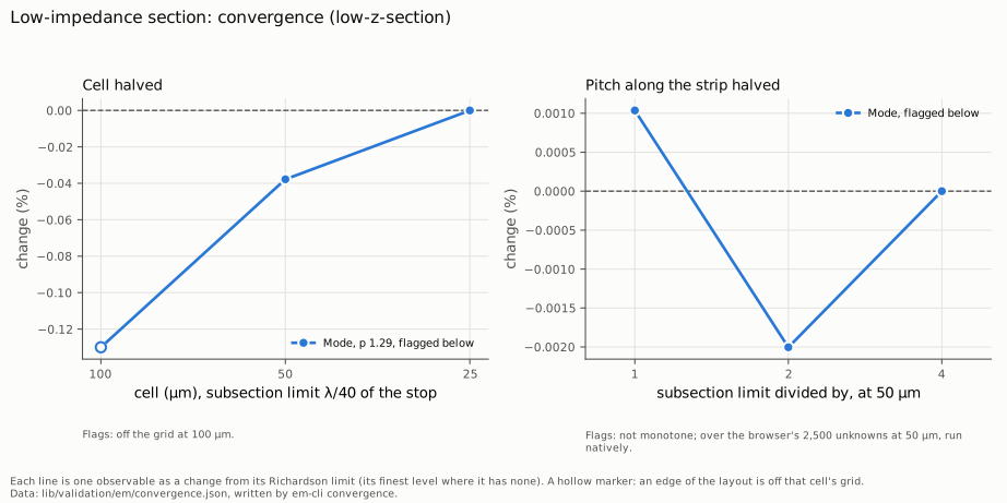
    Mode on 100, 50 and 25 µm cells: 3.3547 GHz, 3.3578 GHz and 3.3591 GHz. No Richardson limit is given, because an edge of the layout is off the 100 µm grid and the mesher rounds it. The levels span 0.13%. Convergence plot

  11. Stepped-impedance resonator

    Geometry
    10 mm of 1.5 mm line, then 10 mm of 0.75 mm line to an open end, the first zero of Im Zin.
    Reference
    openEMS of the same closed box (finest of four meshes, within 0.05% of the next), and a hand value from the box lines, the Garg and Bahl step and the open-end fit.
    Box and cell
    25 by 12.5 mm, lid 8.8 mm, 50 µm, stop 2.4 GHz, 460 unknowns
    • Resonance, openEMS: ours 2.297 GHz, reference 2.292 GHz, error +0.22%, gate within 1%, pass
    • Resonance, hand: ours 2.297 GHz, reference 2.293 GHz, error +0.18%, gate within 1.5%, pass

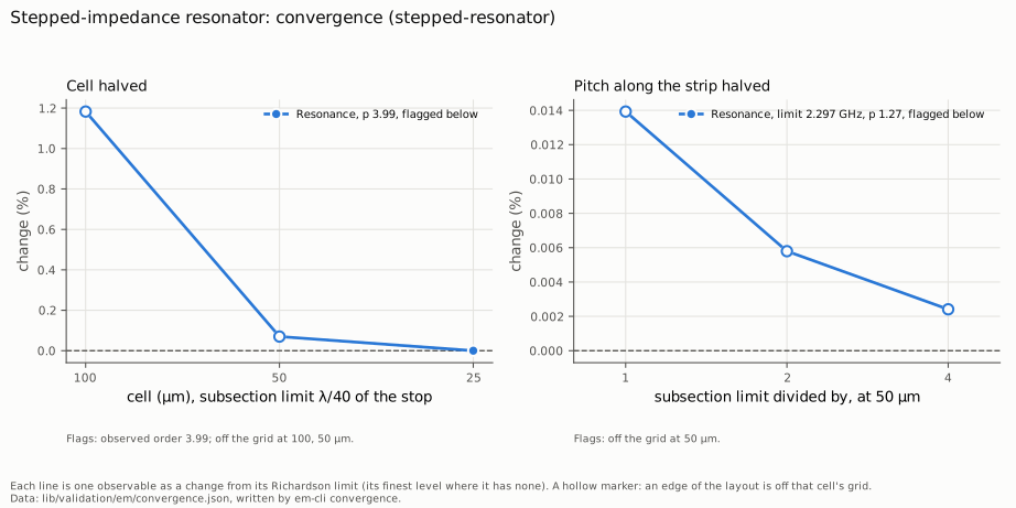
    Resonance on 50 µm cells with the subsection length divided by 1, 2 and 4: 2.2973 GHz, 2.2971 GHz and 2.2970 GHz. Richardson limit 2.2970 GHz, observed order 1.27 where about 2 is expected. At 100 and 50 µm an edge of the layout is off the cell grid and the mesher rounds it, so the cell sizes also change the geometry. Convergence plot

  12. Wide section away from the wall

    Geometry
    A 4 mm wide, 6 mm long section 3 mm from each port wall on 1.5 mm feeds, S from 1 to 7 GHz.
    Reference
    openEMS of the same channel with no end wall at all, so neither its port nor ours enters. The number is the largest complex difference of S.
    Box and cell
    12 by 12 mm, lid 8.8 mm, 100 µm, stop 15 GHz, 2139 unknowns
    • Largest |ΔS|: ours 0.0105, gate under 0.012, pass

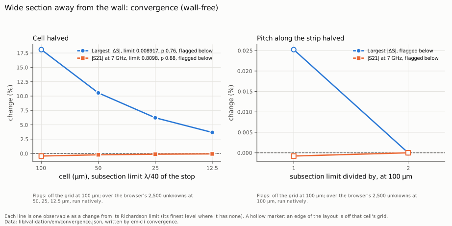
    Largest |ΔS| on 100, 50, 25 and 12.5 µm cells: 0.01053, 0.009858, 0.009472 and 0.009244. Richardson limit 0.008917, observed order 0.76 where about 1 is expected. At 100 µm an edge of the layout is off the cell grid and the mesher rounds it, so that level also changes the geometry. Convergence plot
Question or a correction on an EM case? Send it with the case name.

Attenuator Pad Calculator

Attenuator pads against scikit-rf

Checked
153 pads: pi, T, bridged-T and minimum-loss, exact and built from E24 and E96 parts, 45 of them between unequal impedances. 486 resistor values and 612 S-parameters (S11, S21, S22 and S12).
Reference
A Python script works each pad from the textbook equations in its own code, snaps it to E24 and E96 with its own tables, and builds the resistors as a scikit-rf 2.2.0 circuit. The test never computes an expected value with the calculator's code.
Tolerance
Each exact resistor within 10⁻¹⁰ relative, each E24 or E96 part equal, and each S-parameter within 10⁻¹² absolute.
Result
153 of 153 pads match.
Does not cover
Ideal resistors between real port impedances. Part parasitics and layout are outside it. Power per resistor is checked against hand values in a separate test, not counted here.
Test files
  • lib/pad/skrf-reference.json
  • lib/pad/skrf-reference.py
  • lib/pad/__tests__/skrf.test.ts

Stability Circles

Stability K, μ and stability circles against scikit-rf

Checked
K, |Δ|, μ, μ′ and the load and source stability circles at 83 frequency points: 6 typed cases, the same cases with the ports swapped, and a FET file at 71 points. At 644 test points either side of the boundaries, the stable side is checked against |Γ_in| or |Γ_out| worked straight from S.
Reference
scikit-rf 2.2.0 (Network.stability and stability_circle) for K and the circles, and numpy for Δ, μ and μ′, which scikit-rf does not provide. The 6 typed cases also have hand values in exact fractions.
Tolerance
Within 10⁻⁹, relative where the value is above 1, and 10⁻¹² for the hand values.
Result
83 of 83 frequency points match, and every test point falls on the side the circle says.
Does not cover
Two-port stability at the frequencies in the file. Stability between file points, and oscillation through bias networks or package parasitics the file does not include, are outside it.
Test files
  • lib/stability/stability-reference.json
  • scripts/stability-reference.py
  • lib/stability/__tests__/stability.test.ts

Amplifier Design

Amplifier gains and noise against scikit-rf

Checked
Γ_in and Γ_out at 50 source and load terminations over 5 operating points, and G_T, G_P, G_A and mismatch at each stable one. The gain limit at every point, the conjugate match where one exists, and the noise factor at 40 source terminations over 4 of the points.
Reference
scikit-rf 2.2.0: an ideal lossless network on each side of the 2-port, with every gain read off the cascade in linear watts, so no gain formula is used. Noise from the admittance form, and scikit-rf's own noise figure for the FET file.
Tolerance
Every gain and the noise factor within 10⁻⁹, relative where the value is above 1, and Γ within 10⁻⁹ in |ΔΓ|.
Result
5 of 5 operating points match at every termination.
Does not cover
One bias point at one frequency, small signal, with ideal lossless matching networks. Compression, IP3 and the bias network are outside it.
Test files
  • lib/amplifier/amplifier-reference.json
  • scripts/amplifier-reference.py
  • lib/amplifier/__tests__/gains.test.ts
  • lib/amplifier/__tests__/noise.test.ts

Smith Chart & Matching

Hand-built matching chains against scikit-rf

Checked
4 hand-built chains at 12 frequency points: series L and shunt C onto a complex load, finite-Q parts with resistors, a line with a shorted stub, and a chain of 8 parts, the most the page takes. S11, S21, S12, S22 and Γin, each at two effective permittivities.
Reference
scikit-rf 2.2.0 building each chain from its own media classes and cascading it with its own ** operator. Its answers are saved once and committed.
Tolerance
Each complex value within 10⁻⁹ relative.
Result
4 of 4 chains match at every point.
Does not cover
The hand-build chain. The L-network, stub and quarter-wave solvers are checked against hand values in their own tests, not counted here. Part parasitics beyond a fixed Q are outside it.
Test files
  • lib/match/__tests__/hand-build-skrf-reference.json
  • scripts/match-hand-build-skrf-reference.py
  • lib/match/__tests__/hand-build.test.ts

Coax Loss Calculator

Coax SWR at the radio against scikit-rf

Checked
42 cases: a matched line with 0.1 to 10 dB of loss onto antennas from VSWR 1.1 to 10, at 7 load phases. |Γ| at the antenna and at the radio, the VSWR the radio reads, and the antenna VSWR worked back from that reading.
Reference
scikit-rf 2.2.0: a matched lossy line with the stated loss, cascaded onto each load. Its answers are saved once and committed.
Tolerance
|Γ| and VSWR within 10⁻¹², relative where the value is above 1, and the antenna VSWR worked back within 10⁻⁹.
Result
42 of 42 cases match.
Does not cover
The SWR readout for a line of known loss. Each cable's loss comes from a fit to its datasheet rows; the fits and their residuals are in the dataset at the end of this page. A line whose impedance differs from the radio's is outside it.
Test files
  • lib/coax/radio-swr-skrf-reference.json
  • scripts/coax-radio-swr-skrf-reference.py
  • lib/coax/__tests__/radio-swr.test.ts

Spur Chart

Mixer spur products against exact fractions

Checked
4 frequency plans up to order 6: every output product |m·fRF ± n·fLO| (128 in all) and every input spur that converts into the IF (107), each with its band edges, its centre and whether it lands in band.
Reference
A Python script that imports no site code and works every product and spur in exact fractions, then checks each spur forward through its own equation. It refuses a plan where a band edge only touches another.
Tolerance
Band edges and centres within 10⁻¹² relative; in-band flags exact.
Result
128 of 128 products and 107 of 107 spurs match.
Does not cover
Frequencies and band overlap. Spur levels come from the datasheet table you paste, and filter rejection on the Cascade page from each filter's curve; neither is counted here.
Test files
  • lib/cascade/__tests__/fixtures/spur-reference.json
  • scripts/spur-reference.py
  • lib/cascade/__tests__/spurs.test.ts

Phase Noise to Jitter

Phase noise to jitter against numerical integration

Checked
5 phase noise masks, flat and sloped, with band limits on and between mask points: the integrated phase noise, the phase variance, rms phase error in radians and degrees, jitter, EVM floor and ADC SNR limit (35 values).
Reference
A Python script that imports no site code reads each mask by straight-line interpolation on log offset and integrates it with scipy quad at 10⁻¹³ relative. It never uses the power-law closed form the page uses.
Tolerance
Every value within 10⁻⁹ relative.
Result
35 of 35 values match.
Does not cover
The integral of the mask as typed. How closely the straight lines between points follow the real oscillator, spurs on its phase noise plot, and the ADC's own aperture jitter are outside it.
Test files
  • lib/cascade/__tests__/fixtures/phase-noise-reference.json
  • scripts/phase-noise-reference.py
  • lib/cascade/__tests__/phase-noise-reference.test.ts

Op-Amp Lab

Op-Amp Lab templates against closed forms

Checked
All 8 templates run through the engine the page uses: the operating point, both ends of the DC sweep, and the Bode magnitude and phase at two frequencies.
Reference
Each template's closed form worked by hand, with the op-amp's finite open-loop gain and gain-bandwidth, typed in the test. Never an engine run.
Tolerance
Voltages within 10⁻⁹ V, relative above 1 V, Bode magnitude within 10⁻⁹ dB, and phase within 10⁻⁷°.
Result
8 of 8 templates match.
Does not cover
An op-amp with finite gain and one pole. Slew rate and noise are outside it.
Test files
  • lib/opamp/__tests__/templates.test.ts

dB Power Converter

dB ratio table against hand values

Checked
10 ratios from 0.1 to 1000, in power and in voltage: 20 dB values in the ratio table.
Reference
Worked on paper from the logarithms of 2, 3 and 7, never by running the converter.
Tolerance
Each value within 5 × 10⁻¹⁰ dB of the hand value.
Result
20 of 20 values match.
Does not cover
The ratio table. The dBm, dBµV and antenna-gain conversions have their own hand-value tests, not counted here.
Test files
  • lib/tools/__tests__/db-ratio-table.test.ts

The coax loss fits for all 24 cables, with each fit's residual and datasheet, are free to reuse under CC BY 4.0: CSV, JSON.

Found a number that disagrees with your hand math? Send it with your inputs.